Glossary
2
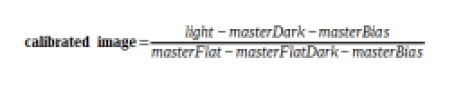
The pre-processing operation consists of calculating the following equation:

This allows the images to be calibrated by removing some of the unwanted signal.
In principle, 3 images are necessary:
The master bias, the master dark and the master flat.
The possibility of optimising the master dark is offered (a multiplier coefficient is applied to the master dark in order to minimise the noise induced by the subtraction of the latter) as well as the correction of deviant pixels.
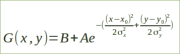
- 2D Gaussian

- 2D Gaussian
A
- ADU
Analog Digital Unit Binary Number Digital Count
There are several concepts and issues going on here that are getting mixed together.
First the ADC
An ADC (Analog To Digital Convertor) takes signal values in a certain range and converts then to a digital number. Let's run some numbers:
A N bit ADC will be able to represent 2^N states. So a 4 bit ADC can represent 16 distinct states, 8 bits => 256 States and a 12 bit convertor will give you 4096 states. By itself that tells you nothing, you need to know that going from a digital representation of say 533 -> 534 means that the input signal changed by certain amount. To keep the example simple I'm going to say that I have an input range from 0 Volts to 4.095 Volts on a 12 bit convertor, that means that when I have a digital number of 0 then I must have had 0 on the input. Let's also assume everything is ideal for now. With my sneaky choice of input range you can see that for every change in the ADC output digital number by one count then the input must have changed by 1 mV.
Why did I pick 4.095? Well a 12 bit convertor will have 4096 digital values that range from 0 to 4095 (2^N-1 when all the bits are set to "1"). So 4.095 Volts/4095 = 1 mv/count. That means that if you have a 3.567 Volt value on the output and it changes to 3.568 Volts ( 1 mV change on the input) then the digital number on the output should change from 3567 to 3568 digital number on the output from 110111101111 to = 110111110000 in raw binary.
Each of these binary steps are called an ADU (Analog Digital Unit) or Binary Number or Digital Count etc. etc. to keep it separate from the number of bits that the ADC has. This is to ensure that the relationship is in a linear range. If you start using "bits" then it is in a logarithmic range (2^N). The main reason these other names/units are used is that LSB's used to be used. What is a LSB? - it stands for Least Significant Bit, i.e. the zeroth bit in the digital number, which changes precisely in step with the ADU but using LSB (and the implied 'bit") is confusing. Imagine saying, " the ADC changed by 30 LSB's therefore the light flux must have changed by 3000 photons ". 30 LSB's really doesn't make sense, it is a mixing of terminology, so people are moving away from that. But that has meant that many different terms being used instead confusing again...
So you have a conversion from voltage into a digital number.
But you are collecting photons, where does voltage come from?
Next the Voltage conversion
All image sensors at some point in the signal chain will convert the collected signal charge into voltage to interact with the outside world. This is always done using a capacitance and a buffer amplifier. This capacitor and the gain of the amplifier set the conversion from electrons into voltage as A/C_sense which is derived from the Q= CV equation. With C_sense = the sense node capacitance and A = gain of the buffer amplifier.
Next the photon conversion
When a Photon comes rattling into a pixel it has to make it into the photosensitive substrate, this interface is controlled by the fresnel equations and dictates how much light goes into the substrate based upon the indices of refraction and the various materials and AR coatings present (AR = Anti-reflection). This is known as the external QE (Quantum efficiency). Once in the substrate the photons are absorbed through it is depth and generate electron/hole pairs through the photo electron effect. Electric fields sweep the carriers into storage structures. The absorption depth and the depth of influence of the electric fields (these two depths may not be co-incident) are what determines the Internal QE. NOt every converted photon's carriers get collected.
These collected carriers (either electrons or holes) are brought to the sense node and converted into voltages. Where this conversion happens (carrier to voltage) is determined by the type of sensor, a CCD or CMOS image sensor.
The total conversion process;
(Photon flux) * (Integration period) * QE_external *QE_Internal * A/C_sense * ADC_conversion Will give you units of Photons/ADU. (1)
- Asinh
The inverse hyperbolic sine is commonly used, it reproduces the perceptive capacity of the human eye, allowing to perceive significantly different brightness levels simultaneously. The asinh function is close to the logarithmic mode but has a better behavior around zero.

- Asinh
The inverse hyperbolic sine is commonly used, it reproduces the perceptive capacity of the human eye, allowing to perceive significantly different brightness levels simultaneously. The asinh function is close to the logarithmic mode but has a better behavior around zero.
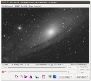
- AutoStretch
Siril performs auto stretching curves to adjust the image and make it visible on the screen.
B-C
- Banding
Phenomenon manifested as horizontal bands of darker than the rest of the image. This defect is easily visible on a plain and clear background.
- Bias
offset
A BIAS image is an image taken in total darkness (cap closed) and at the fastest speed.
In practice, on modern SLR cameras, this corresponds to a speed of 1/4000s.
The BIAS will contain the electronic noise as well as the readout signal from the camera.
- CFA
Color Filter Array
The CFA image is a black and white image that shows the signal received by each pixel of the sensor.
The pixels are alternately covered with red filters, green and blue.
In general, there are twice as many green pixels than red and blue (the case of the Bayer matrix). For example, if the observed object is uniformly red, only the red pixels will be illuminated.
This term is often used to describe one-channel image content of a color image, with each pixel corresponding to values acquired behind an on-sensor filter.
This is to oppose to debayer images (or debayered or demosaiced).
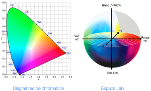
- CIE L*a*b*
CIELAB
CIE L*a*b*, often abbreviated CIELAB is a color space for surface colors.
- The component L* is clarity, which ranges from 0 (black) to 100 (white).
- The component a* represents a range of 600 levels on a red pin (299 positive) → green (-300 negative value) via the gray (0).
- The component b* represents a range of 600 levels on a yellow axis (299 positive) → blue (negative value -300) through the gray (0).
- cut
CutInstead of keeping pixels with values greater than the value "hi" white when checked: displays black pixels when saturated

D-E
- Darks
The darks are taken with the same exposure time and ISO as the images to be pre-processed, but in the dark.
- Drizzle
Drizzle is a simple algorithm that creates an image that is larger than the images in the stack and interpolates between pixels to ensure it reproduces fine detail in edges despite the effects of stacking transformations.
- Dynamic PSF
Dynamic PSF is a dynamic tool inspired by the PixInsight routine of the same name. It is used to fit unsaturated stars within the image.
- Enhanced Correlation Coefficient Maximization
This is an algorithm dedicated to the planet surfaces taken from opencv 3.0
- Equalisation of CFA flats
Greyflat
A small region is taken in the centre of the CFA flat and the average of each channel is made.
F-G
- Flat
An optical instrument does not illuminate the sensor evenly. In addition, dust on the sensor can lead to the appearance of spots on the images. To correct these effects, we need to divide each image by a masterFlat. The masterFlat is obtained from the median (or average with deviant pixels rejected) combination of images of a uniform light area (usually the background sky at dusk or dawn), taken with a short exposure time
- FWHM
Full-Width Half-Maximum
The technical term Full-Width Half-Maximum
FWHM, is used to describe a measurement of the width of a star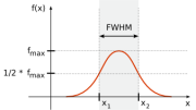
It is a well-defined number which can be used to compare the quality of images obtained under different observing conditions. In an astronomical image, the FWHM is measured for a selection of stars in the frame and the "seeing" or image quality is reported as the mean value. Solower value for FWHM is better.
With Siril it's possible to obtain the FWHM parameters in arcseconds units. This requires you fill all fields corresponding to your camera and lens/telescope focal in the setting parameter window. If standard FITS keywords FOCALLEN, XPIXSZ, YPIXSZ, XBINNING and YBINNING are read in the FITS HDU, the PSF will also compute the image scale in arcseconds per pixel.
- FWHM
Full-Width Half-Maximum
The technical term Full-Width Half-Maximum
FWHM, is used to describe a measurement of the width of a star
It is a well-defined number which can be used to compare the quality of images obtained under different observing conditions. In an astronomical image, the FWHM is measured for a selection of stars in the frame and the "seeing" or image quality is reported as the mean value. Solower value for FWHM is better.
With Siril it is possible to obtain the FWHM parameters in arcseconds units. This requires you fill all fields corresponding to your camera and lens/telescope focal in the setting parameter window. If standard FITS keywords FOCALLEN, XPIXSZ, YPIXSZ, XBINNING and YBINNING are read in the FITS HDU, the PSF will also compute the image scale in arcseconds per pixel.
- Generalized Extreme Studentized Deviate Test
GESDT
H-K
- Histogramme
The histogram equalization increases the contrast of the image by increasing the dynamic range of the intensity given to the pixels with the most likely intensity values.
It is highly recommended to evaluate all the signals contained in the image.
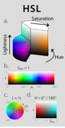
- HSL
HLS
stands for hue, saturation, and lightness (or luminosity), and is also often called HLS
- Hue
- saturation
- luminance
- HSV
HSB
The HSV, or HSB, model describes colors in terms of hue, saturation, and value (brightness).

L
- Lanczos4
"Lanczos resampling and Lanczos filtering are two applications of a mathematical formula. It can be used as a low-pass filter or used to smoothly interpolate the value of a digital signal between its samples. In the latter case it maps each sample of the given signal to a translated and scaled copy of the Lanczos kernel, which is a sinc function windowed by the central lobe of a second, longer, sinc function. The sum of these translated and scaled kernels is then evaluated at the desired points.
Lanczos resampling is typically used to increase the sampling rate of a digital signal, or to shift it by a fraction of the sampling interval. It is often used also for multivariate interpolation, for example to resize or rotate a digital image. It has been considered the "best compromise" among several simple filters for this purpose"(1)
- linear
the default mode of Siril. The pixels are displayed from dark to light in a linear scale.
- Linear Fit Clipping
It fits the best straight line (y=ax+b) of the pixel stack and rejects outliers. This algorithm performs very well with large stacks and images containing sky gradients with differing spatial distributions and orientations.
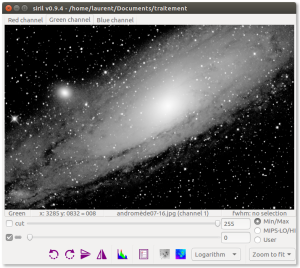
- Logarithm
The logarithmic scale. The operation simultaneously exacerbating the weak and light levels of the image.
M
- Median MAD clipping
It is similar to the sigma clipping except the median absolute deviation (MAD) is used instead of the standard deviation to compute the rejection bounds around the median of the stack.
- Median Sigma Clipping
This is the same algorithm as
Sigma Clippingexcept than the rejected pixels are replaced by the median value of the stack.- Median Stacking
This method is mostly used for dark/flat/offset stacking. The median value of the pixels in the stack is computed for each pixel. As this method should only be used for dark/flat/offset stacking, it does not take into account shifts computed during registration. The increase in SNR is proportional to 0.8√N.
- Minimization
Minimization is performed with a non-linear Levenberg-Marquardt algorithm thanks to the very robust GNU Scientific Library.
As a first step, the algorithm runs a set of parameters excluding rotation angle in order to set good start values and thus, avoiding possible divergence. If σx−σy>0.01 (parameters directly computed in the 2-D Gaussian formula, see above), then another fit is run with the angle parameter.
Therefore, the Siril Dynamic PSF provides accurate values for all the fitted parameters.
N-R
- Normalisation
Normalisation matches the mean background of all input images, then, the normalisation is processed by multiplication or addition. Keep in mind that both
processes generally lead to similar results but multiplicative normalisation is prefered for image which will be used for multiplication or division as flat-field.
- Scale matches dispersion by weighting all input images. This tends to improve the signal-to-noise ratio and therefore this is the option used by default with
the additive normalisation.
The offset and dark masters should not be processed with normalisation.
However, multiplicative normalisation must be used with flat-field frames.
- Percentile Clipping
This is a one step rejection algorithm ideal for small sets of data (up to 6 images).
- Pixel Maximum Stacking
This algorithm is mainly used to construct long exposure star-trails images. Pixels of the image are replaced by pixels at the same coordinates if intensity is greater.
- Pixel Minimum Stacking
This algorithm is mainly used for cropping sequence by removing black borders. Pixels of the image are replaced by pixels at the same coordinates if intensity is lower.
- Registration
Registration is basically aligning the images from a sequence to be able to process them afterwards.
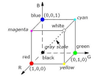
- RGB
RVB
RGB (red, green, and blue) refers to a system for representing the colors to be used on a computer display. Red, green, and blue can be combined in various proportions to obtain any color in the visible spectrum. Levels of R, G, and B can each range from 0 to 100 percent of full intensity. Each level is represented by the range of decimal numbers from 0 to 255 (256 levels for each color), equivalent to the range of binary numbers from 00000000 to 11111111, or hexadecimal 00 to FF. The total number of available colors is 256 x 256 x 256, or 16,777,216 possible colors.
S-Z
- setmag
setmag magnitude
Defines the magnitude constant by selecting a star and giving the true magnitude. All PSF computations will return the true magnitude after this command.
- setmagseq
setmagseq magnitude
This command is only valid after having run
seqpsfor its graphical counterpart (select the area around a star and launch thepsf analysisfor the sequence, it will appear in the graphs).- Sigma Clipping
This is an iterative algorithm which will reject pixels whose distance from median will be farthest than two given values in sigma units(σlow, σhigh).
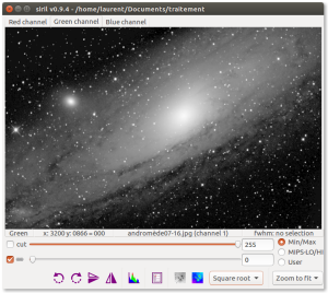
- Square root
The square root of each pixel. This can be seen primarily in this mode are the brightest parts of the image.
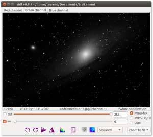
- Squared
Square of each pixel. Which can be seen with this model viewer is primarily the most brightest part of the image.
- Sum Stacking
This is the simplest algorithm: each pixel in the stack is summed. The increase in signal-to-noise ratio (SNR) is proportional to √N, where N is the number of images. Because of the lack of normalization and rejection, this method should only be used for planetary processing.
- Winsorized Sigma Clipping
This is very similar to Sigma Clipping method Sigma Clipping